Matching model and selection correction for group formation

The function provides a Gibbs sampler for a structural matching model that estimates preferences and corrects for sample selection bias when the selection process is a one-sided matching game; that is, group/coalition formation.

The input is individual-level data of all group members from one-sided matching marktes; that is, from group/coalition formation games.

In a first step, the function generates a model matrix with characteristics of all feasible groups of the same size as the observed groups in the market.

For example, in the stable roommates problem with \(n=4\) students \(\{1,2,3,4\}\) sorting into groups of 2, we have \( {4 \choose 2}=6 \) feasible groups: (1,2)(3,4) (1,3)(2,4) (1,4)(2,3).

In the group formation problem with \(n=6\) students \(\{1,2,3,4,5,6\}\) sorting into groups of 3, we have \( {6 \choose 3} =20\) feasible groups. For the same students sorting into groups of sizes 2 and 4, we have \( {6 \choose 2} + {6 \choose 4}=30\) feasible groups.

The structural model consists of a selection and an outcome equation. The Selection Equation determines which matches are observed (\(D=1\)) and which are not (\(D=0\)). $$ \begin{array}{lcl} D &= & 1[V \in \Gamma] \\ V &= & W\alpha + \eta \end{array} $$ Here, \(V\) is a vector of latent valuations of all feasible matches, ie observed and unobserved, and \(1[.]\) is the Iverson bracket. A match is observed if its match valuation is in the set of valuations \(\Gamma\) that satisfy the equilibrium condition (see Klein, 2015a). This condition differs for matching games with transferable and non-transferable utility and can be specified using the method argument. The match valuation \(V\) is a linear function of \(W\), a matrix of characteristics for all feasible groups, and \(\eta\), a vector of random errors. \(\alpha\) is a paramter vector to be estimated.

The Outcome Equation determines the outcome for observed matches. The dependent variable can either be continuous or binary, dependent on the value of the binary argument. In the binary case, the dependent variable \(R\) is determined by a threshold rule for the latent variable \(Y\). $$ \begin{array}{lcl} R &= & 1[Y > c] \\ Y &= & X\beta + \epsilon \end{array} $$ Here, \(Y\) is a linear function of \(X\), a matrix of characteristics for observed matches, and \(\epsilon\), a vector of random errors. \(\beta\) is a paramter vector to be estimated.

The structural model imposes a linear relationship between the error terms of both equations as \(\epsilon = \delta\eta + \xi\), where \(\xi\) is a vector of random errors and \(\delta\) is the covariance paramter to be estimated. If \(\delta\) were zero, the marginal distributions of \(\epsilon\) and \(\eta\) would be independent and the selection problem would vanish. That is, the observed outcomes would be a random sample from the population of interest.

stabit(x, m.id = "m.id", g.id = "g.id", R = "R", selection = NULL,
  outcome = NULL, simulation = "none", seed = 123, max.combs = Inf,
  method = "NTU", binary = FALSE, offsetOut = 0, offsetSel = 0,
  marketFE = FALSE, censored = 0, gPrior = FALSE, dropOnes = FALSE,
  interOut = 0, interSel = 0, standardize = 0, niter = 10,
  verbose = FALSE)

Arguments

x	data frame with individual-level characteristics of all group members including market- and group-identifiers.
m.id	character string giving the name of the market identifier variable. Defaults to "m.id".
g.id	character string giving the name of the group identifier variable. Defaults to "g.id".
R	dependent variable in outcome equation. Defaults to "R".
selection	list containing variables and pertaining operators in the selection equation. The format is operation = "variable". See the Details and Examples sections.
outcome	list containing variables and pertaining operators in the outcome equation. The format is operation = "variable". See the Details and Examples sections.
simulation	should the values of dependent variables in selection and outcome equations be simulated? Options are "none" for no simulation, "NTU" for non-transferable utility matching, "TU" for transferable utility or "random" for random matching of individuals to groups. Simulation settings are (i) all model coefficients set to alpha=beta=1; (ii) covariance between error terms delta=0.5; (iii) error terms eta and xi are draws from a standard normal distribution.
seed	integer setting the state for random number generation if simulation=TRUE.
max.combs	integer (divisible by two) giving the maximum number of feasible groups to be used for generating group-level characteristics.
method	estimation method to be used. Either "NTU" or "TU" for selection correction using non-transferable or transferable utility matching as selection rule; "outcome" for estimation of the outcome equation only; or "model.frame" for no estimation.
binary	logical: if TRUE outcome variable is taken to be binary; if FALSE outcome variable is taken to be continuous.
offsetOut	vector of integers indicating the indices of columns in X for which coefficients should be forced to 1. Use 0 for none.
offsetSel	vector of integers indicating the indices of columns in W for which coefficients should be forced to 1. Use 0 for none.
marketFE	logical: if TRUE market-level fixed effects are used in outcome equation; if FALSE no market fixed effects are used.
censored	draws of the delta parameter that estimates the covariation between the error terms in selection and outcome equation are 0:not censored, 1:censored from below, 2:censored from above.
gPrior	logical: if TRUE the g-prior (Zellner, 1986) is used for the variance-covariance matrix.
dropOnes	logical: if TRUE one-group-markets are exluded from estimation.
interOut	two-colum matrix indicating the indices of columns in X that should be interacted in estimation. Use 0 for none.
interSel	two-colum matrix indicating the indices of columns in W that should be interacted in estimation. Use 0 for none.
standardize	numeric: if standardize>0 the independent variables will be standardized by dividing by standardize times their standard deviation. Defaults to no standardization standardize=0.
niter	number of iterations to use for the Gibbs sampler.
verbose	.

Details

Operators for variable transformations in selection and outcome arguments.

add

sum over all group members and divide by group size.

int

sum over all possible two-way interactions \(x*y\) of group members and divide by the number of those, given by choose(n,2).

ieq

sum over all possible two-way equality assertions \(1[x=y]\) and divide by the number of those.

ive

sum over all possible two-way interactions of vectors of variables of group members and divide by number of those.

inv

...

dst

sum over all possible two-way distances between players and divide by number of those, where distance is defined as \(e^{-|x-y|}\).

References

Klein, T. (2015a). Does Anti-Diversification Pay? A One-Sided Matching Model of Microcredit. Cambridge Working Papers in Economics, #1521.

Zellner, A. (1986). On assessing prior distributions and Bayesian regression analysis with g-prior distributions, volume 6, pages 233--243. North-Holland, Amsterdam.

Examples

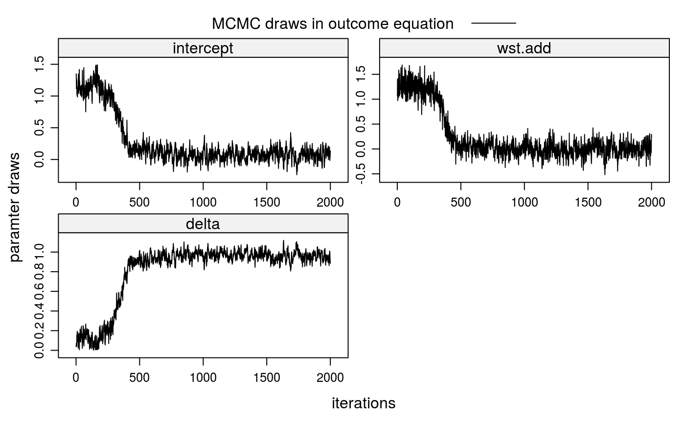
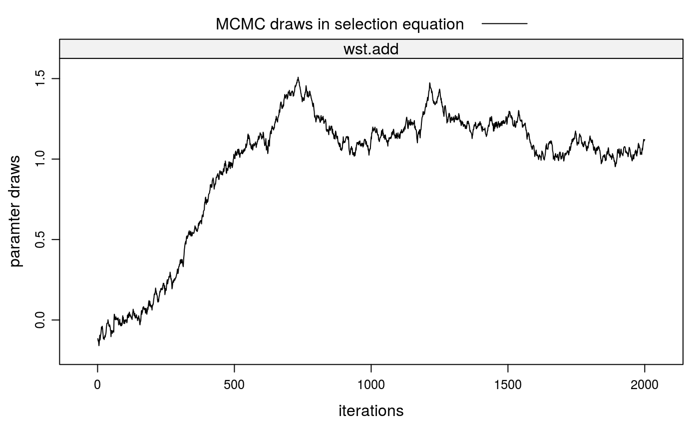
##\dontrun{
## --- SIMULATED EXAMPLE ---

## 1. Simulate one-sided matching data for 200 markets (m=200) with 2 groups
##    per market (gpm=2) and 5 individuals per group (ind=5). True parameters 
##    in selection equation is wst=1, in outcome equation wst=0. 

## 1-a. Simulate individual-level, independent variables
 idata <- stabsim(m=200, ind=5, seed=123, gpm=2)
 head(idata)
#>   m.id g.id         wst  R
#> 1    1    1 -0.56047565 NA
#> 2    1    1 -0.23017749 NA
#> 3    1    1  1.55870831 NA
#> 4    1    1  0.07050839 NA
#> 5    1    1  0.12928774 NA
#> 6    1    2  1.71506499 NA

## 1-b. Simulate group-level variables 
 mdata <- stabit(x=idata, simulation="NTU", method="model.frame",
 selection = list(add="wst"), outcome = list(add="wst"), verbose=FALSE)
#> Generating group-level data for 200 markets... 
 head(mdata$OUT)
#>   m.id g.id intercept    wst.add          R         xi    epsilon
#> 1    1    1         1  0.3698086  1.5670690 -0.8497043  1.5670690
#> 2    1    2         1 -0.2205573 -2.4953827 -1.1373036 -2.4953827
#> 3    2    1         1  0.7198747  1.3680982 -1.1198997  1.3680982
#> 4    2    2         1 -0.3026307  0.3707344 -0.7822018  0.3707344
#> 5    3    1         1 -0.3271234  3.0184259 -0.3719449  3.0184259
#> 6    3    2         1 -0.5219943 -0.1015002 -0.6527744 -0.1015002
 head(mdata$SEL)
#>   m.id g.id reg.id    wst.add D          V         eta
#> 1    1    1      2  0.3698086 1  2.7865819  2.41677335
#> 2    1    2      1 -0.2205573 1 -1.5786364 -1.35807906
#> 3    1    3    128  0.1935703 0 -0.1503470 -0.34391723
#> 4    1    4    129  0.2221432 0  1.8206520  1.59850877
#> 5    1    5    130  0.3377849 0  0.2492198 -0.08856511
#> 6    1    6    131  0.3860231 0  1.4668226  1.08079950


## 2. Bias from sorting

## 2-a. Naive OLS estimation
 lm(R ~ wst.add, data=mdata$OUT)$coefficients
#> (Intercept)     wst.add 
#>    1.321692    1.281722 

## 2-b. epsilon is correlated with independent variables
 with(mdata$OUT, cor(epsilon, wst.add))
#> [1] 0.3650137

## 2-c. but xi is uncorrelated with independent variables
 with(mdata$OUT, cor(xi, wst.add))
#> [1] 0.001335074

## 3. Correction of sorting bias when valuations V are observed

## 3-a. 1st stage: obtain fitted value for eta
lm.sel <- lm(V ~ -1 + wst.add, data=mdata$SEL)
lm.sel$coefficients
#>  wst.add 
#> 1.006372 

eta <- lm.sel$resid[mdata$SEL$D==1]

## 3-b. 2nd stage: control for eta
 lm(R ~ wst.add + eta, data=mdata$OUT)$coefficients
#> (Intercept)     wst.add         eta 
#>  0.09072970  0.09468869  0.94626877 


## 4. Run Gibbs sampler
 fit1 <- stabit(x=idata, method="NTU", simulation="NTU", censored=1,
                selection = list(add="wst"), outcome = list(add="wst"),
                niter=2000, verbose=FALSE)
#> Generating group-level data for 200 markets... 
#> Drawing 2000 MCMC samples...


## 5. Coefficient table
 summary(fit1)
#> 
#> Coefficients for multi-index sample selection model.
#> Method: Klein (2015), one-sided matching market
#> 
#> Call:
#> stabit(x = idata, selection = list(add = "wst"), outcome = list(add = "wst"), 
#>     simulation = "NTU", method = "NTU", censored = 1, niter = 2000, 
#>     verbose = FALSE)
#> 
#> Selection equation:
#>         Estimate  StdErr t.value  p.value   
#> wst.add  1.15188 0.41565  2.7713 0.005846 **
#> 
#> Outcome equation:
#>             Estimate     StdErr t.value p.value   
#> intercept  0.0733179  0.3871956  0.1894 0.84991   
#> wst.add   -0.0083934  0.4812529 -0.0174 0.98609   
#> delta      0.9632351  0.2999799  3.2110 0.00143 **
#> ---
#> Signif. codes:  0 '***' 0.001 '**' 0.01 '*' 0.05 '.' 0.1 ' ' 1


## 6. Plot MCMC draws for coefficients
 plot(fit1)
##}

# NOT RUN {
## --- REPLICATION, Klein (2015a) ---

## 1. Load data 
 data(baac00); head(baac00)

## 2. Run Gibbs sampler
 klein15a <- stabit(x=baac00, selection = list(inv="pi",ieq="wst"),
        outcome = list(add="pi",inv="pi",ieq="wst",
        add=c("loan_size","loan_size2","lngroup_agei")), offsetOut=1,
        method="NTU", binary=TRUE, gPrior=TRUE, marketFE=TRUE, niter=800000)

## 3. Marginal effects
 summary(klein15a, mfx=TRUE)

## 4. Plot MCMC draws for coefficients
 plot(klein15a)
# }